Home

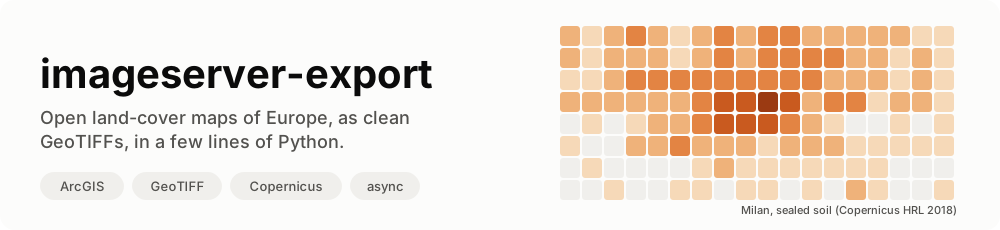
imageserver-export is a small, typed, async Python library that turns an area of any ArcGIS ImageServer into one clean GeoTIFF. Its first use is the open server of the European Environment Agency, which publishes the Copernicus Land Monitoring Service maps of all of Europe, at 10 m: how much of the ground is sealed by concrete and asphalt, how dense the trees are, where the grassland, the water and the wetlands are. No account, no key, no manual download.

async with ImageServer(eea("HRL_ImperviousnessDensity_2018")) as server:
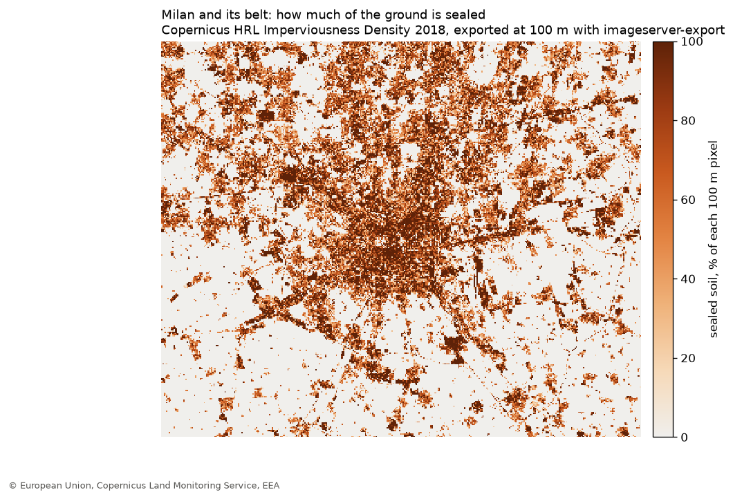
    await server.export(Grid.from_lonlat((8.95, 45.33, 9.45, 45.62), res=100), Path("milan.tif"))

Three dependencies: httpx, numpy, rasterio.

Map of Milan and its belt: the share of sealed soil in each 100 m pixel, from bare fields in light beige to the fully sealed centre in dark brown

What is an ImageServer, in 30 seconds¶

Many public agencies publish their maps with ArcGIS Server. An ImageServer is the part of it that serves rasters: grids of numbers, one per pixel, like satellite-derived land cover. You give it a box, a size and a coordinate system, and its exportImage operation sends back a picture of that box.

That is enough to view a map, but not to use it. One request returns at most a few thousand pixels a side, so Italy at 10 m takes thousands of them. They have to line up exactly, or the pieces shift against each other. And when something goes wrong, the server still answers "200 OK", with an error message where the image should be.

This library does that part for you.

What this library does¶


🗺️	One area, one GeoTIFF	Give it a longitude/latitude box and a resolution; get back one tiled, compressed GeoTIFF, georeferenced in the CRS you chose (LAEA Europe by default).
📐	Pixels that line up	The grid is snapped to whole pixels, and every request is a window of it: the server never resamples to fit, and tiles never shift.
🧩	Big areas in pieces	The area is cut into tiles the server accepts, fetched a few at a time, and pasted as they arrive. A whole country is just more tiles.
🛟	A file or nothing	The mosaic is written to `out.tif.part` and renamed only when every tile is in. A failure leaves nothing a later reader could mistake for a whole map.
🚨	Errors that say why	A JSON error sent with "200 OK", or a tile of the wrong size, stops the export with the server's own message.
🧾	Where it came from	The file carries its own provenance as GeoTIFF tags: service URL, interpolation, valid range, valid pixels, when and with which version. Add your own with `tags=`.
🏷️	What the values mean	`info()` describes the service (pixel type, size, extent, largest image); `attribute_table()` gives the label of every pixel value.
🔌	Your HTTP, your rules	Bring your own `httpx.AsyncClient`, or a `send` function: a shared retry policy, a cache or a rate limiter then sees every request.

Who is it for¶

Researchers and analysts who need a Copernicus Land layer for a region, at the resolution of their own grid, in a script they can run again.
Risk and climate tools that turn land cover into a factor per cell: sealed soil makes rain run off faster, tree cover feeds fires, wetlands change how floods spread.
Anyone with an ArcGIS ImageServer to read, from the EEA or from a regional or national agency: the library is not tied to one server.

It was written for Limen, an open early-warning platform for landslides, floods and wildfires in Italy, which uses sealed soil to amplify the rain-driven flood trigger.

Quick start¶

1. Install¶

pip install imageserver-export

2. Export an area¶

import asyncio
from pathlib import Path

from imageserver_export import Grid, ImageServer, eea


async def main() -> None:
    async with ImageServer(eea("HRL_ImperviousnessDensity_2018")) as server:
        # Milan and its belt, at 100 m, in LAEA Europe (EPSG:3035).
        grid = Grid.from_lonlat((8.95, 45.33, 9.45, 45.62), res=100)
        result = await server.export(grid, Path("milan.tif"), valid_range=(0, 100))
        print(result.width, "x", result.height, "pixels,", f"{result.valid_fraction:.0%} valid")


asyncio.run(main())

valid_range=(0, 100) tells the library which values are real data: this layer uses 254 for "unclassifiable" and 255 for "no data" (the sea, or outside Europe), and both are kept in the file as they are.

3. Read it¶

The result is an ordinary GeoTIFF: open it in QGIS, or read it with rasterio:

import rasterio

with rasterio.open("milan.tif") as src:
    band = src.read(1)
    sealed = band[band <= 100]
    print(f"mean sealed soil: {sealed.mean():.1f} %")  # ~25 % around Milan

The open maps of Europe¶

The EEA serves 26 Copernicus Land layers this way (eea(name) builds the URL, list_services(f"{EEA_URL}/{EEA_FOLDER}") lists them). Among them:

Layer (`eea(...)`)	What each pixel says	Native pixel
`HRL_ImperviousnessDensity_2018`	% of the ground sealed by buildings, roads, car parks	10 m
`HRL_TreeCoverDensity_2018`	% of the ground under tree crowns	10 m
`HRL_DominantLeafType2018`	broadleaved or coniferous forest	10 m
`HRL_Grassland_2018`	grassland or not	10 m
`HRL_WaterWetness_2018`	permanent water, temporary water, wet and dry ground	10 m
`HRL_SmallWoodyFeatures_2018_005m`	hedges, tree rows, small groves	5 m
`HRL_ImperviousnessChange_15_18`	how sealed soil changed, 2015 to 2018	20 m

Each layer has a raster attribute table: await server.attribute_table() returns, for the imperviousness layer, 102 rows such as {"Value": 1, "Class_name": "1% imperviousness value", "Area_km2": 222.19}.

How it works¶

How an export works: an area becomes a grid on whole pixels, the grid is cut into tiles that are requested with exportImage, and the tiles become one GeoTIFF that is renamed from .part only when whole

flowchart LR
    A["Grid.from_lonlat(box, res)"] --> B["plan(grid, tile_px)"]
    B --> C{{"exportImage<br/>per tile, 3 at a time"}}
    C -->|"GeoTIFF bytes"| D["check_image()"]
    C -->|"200 + JSON error"| X["ImageServerError"]
    D --> E["Mosaic.paste()<br/>size checked"]
    E --> F["out.tif.part"]
    F -->|"all tiles in"| G["out.tif"]
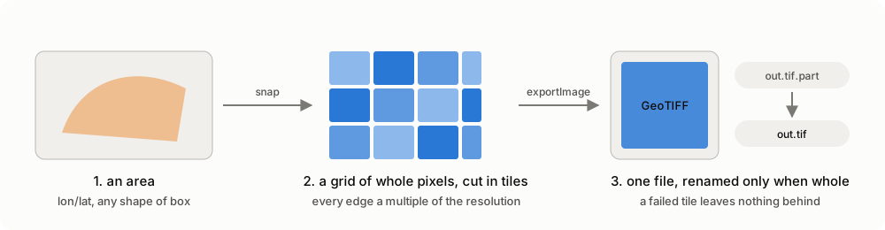
    F -->|"any failure"| H["deleted"]

The grid. Grid.from_lonlat reprojects the box with densified edges (in an equal-area projection the sides of a geographic box curve, and its southern point is not a corner), then grows it outward to whole pixels.
The tiles. plan() covers the grid exactly once, edge tiles clamped to it. Every tile's box is a multiple of the resolution, so the server returns exactly the size asked for, with no resampling.
The requests. export_params() builds each exportImage query in the grid's own CRS, nearest neighbour by default. check_image() turns a JSON answer into an error with the server's message.
The mosaic. Mosaic writes a tiled, deflate-compressed GeoTIFF to .part, refuses a tile whose size differs from the one asked for, counts the valid pixels, writes the provenance tags, and renames the file only on success.

Every step is a plain function or class you can use alone; ImageServer just puts them together.

Why nearest neighbour¶

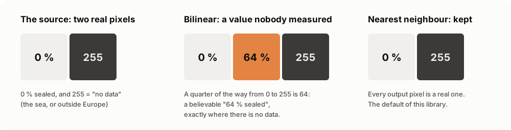
Between a 0 percent pixel and a 255 no-data pixel, bilinear resampling invents a believable 64 percent; nearest neighbour keeps the two real values

Many land-cover layers keep their "no data" marker in the same band as the data: 0 to 100 are percentages, 255 is "nothing here". Bilinear or cubic resampling averages neighbours, so between a 0 % field and a 255 sea pixel it can produce 64: a believable "64 % sealed", exactly where nothing was measured. Nothing downstream can tell it from a real value.

So the default is RSP_NearestNeighbor: every output pixel is one the server really has. Pass interpolation="RSP_BilinearInterpolation" only for continuous layers with no sentinel values.

Recipes¶

Tree cover of a region, at 20 m¶

grid = Grid.from_lonlat((15.3, 39.9, 16.9, 41.2), res=20)  # Basilicata
async with ImageServer(eea("HRL_TreeCoverDensity_2018")) as server:
    await server.export(
        grid,
        Path("basilicata_trees.tif"),
        valid_range=(0, 100),
        on_tile=lambda done, total: print(f"{done}/{total}"),
    )

A whole country, without asking for the sea¶

grid = Grid.from_lonlat((6.6, 35.5, 18.6, 47.1), res=100)  # Italy
async with ImageServer(eea("HRL_ImperviousnessDensity_2018")) as server:
    result = await server.export(
        grid, Path("italy.tif"), valid_range=(0, 100), skip_empty=True, resume=True
    )
print(result.skipped, "of", result.tiles, "tiles were only sea")

skip_empty asks first for one overview, 32 times coarser at the default tile size, and sends no request for a tile with no data on it or next to it: those are filled with "no data". Around Lampedusa it skipped 6 tiles out of 9, with the same pixels as the full export. A feature smaller than one overview pixel and surrounded by sea can be missed, so it is off by default.

resume keeps every tile that arrived in italy.tif.tiles/: if the export fails half way, running it again only asks for the missing ones.

From 100 m pixels to 1 km cells¶

from imageserver_export import aggregate

cells = aggregate(Path("italy.tif"), 10, valid_range=(0, 100))
cells.mean  # mean sealed soil per 1 km cell, NaN where no data
cells.valid_fraction  # share of each cell that held real data
cells.grid  # the 1 km grid, same corner as the raster

Sentinels stay out of the mean: a coastal cell half in the sea is the mean of its land, with valid_fraction 0.5, not 128 % sealed. The raster is read one strip of cells at a time.

Your own grid, in your CRS¶

# Snap to an existing 1 km grid in UTM 32N.
grid = Grid.snap((500_000, 4_500_000, 560_000, 4_560_000), res=1000, crs=32632)

Label the classes¶

async with ImageServer(eea("HRL_WaterWetness_2018")) as server:
    rows = await server.attribute_table()


# The label field is `Class_name` in some layers and `class_name` in others.
def label(row: dict) -> str | None:
    return next((v for k, v in row.items() if k.lower() == "class_name"), None)


labels = {row["Value"]: label(row) for row in rows}
# {0: 'Dry', 1: 'Permanent water', 2: 'Temporary water', 3: 'Permanent wet', ...}

Any other ImageServer¶

server = ImageServer("https://example.org/arcgis/rest/services/Elevation/ImageServer")
info = await server.info()  # pixel type, size, extent, largest image
await server.export(
    Grid.snap(box, res=info.pixel_size[0], crs=3857),
    Path("dem.tif"),
    pixel_type="F32",
    dtype="float32",
    nodata=None,
)

Bring your own HTTP¶

import httpx

async with httpx.AsyncClient(timeout=120) as client:  # your timeouts, proxies
    server = ImageServer(url, client, retries=5)


async def send(method: str, url: str, **kw) -> httpx.Response:
    return await my_retrying_client.request(method, url, **kw)  # your policy


server = ImageServer(url, send=send)  # every request goes through `send`

For AI agents: the MCP server¶

pip install "imageserver-export[mcp]"
claude mcp add imageserver -- imageserver-mcp     # Claude Code

Or in Claude Desktop's claude_desktop_config.json:

{ "mcpServers": { "imageserver": { "command": "imageserver-mcp" } } }

Then ask "how much of the ground is sealed around Milan, and what is the value at the Duomo?". The agent gets six tools:

Tool	What it answers
`list_layers`	the layers of a folder (by default the EEA's 26 Copernicus Land layers)
`describe_layer`	pixel type, native resolution, CRS, extent, and what each value means
`attribute_table`	the raster attribute table, up to `limit` rows
`sample_point`	the value at a longitude/latitude, with its label
`area_summary`	mean, min, max, valid share and class counts (with labels) of a box
`export_area`	writes a box as a GeoTIFF into the output folder (the only tool that writes)

A service is an EEA layer name or the URL of any ImageServer. Every number comes from the library, not from the model: the agent finds the data and explains it, the same rule as in Limen. Areas are capped (4 million pixels for a summary, 25 million for an export) and a refusal says which resolution would fit, so a single call cannot ask a server for a continent at 10 m.

Over HTTP: imageserver-mcp --transport streamable-http --port 8768 serves /mcp, and /health for container healthchecks. Every option also reads an environment variable (IMAGESERVER_MCP_TRANSPORT, _HOST, _PORT, _ALLOWED_HOSTS, _OUTPUT).

Tried live: the Duomo of Milan is 100% imperviousness value; the box of Milan and its belt at 100 m is 27.9 % sealed on average, 59 % of it not sealed at all.

The traps we already fell into¶

"200 OK" is not success. An ImageServer answers a bad request with HTTP 200 and a JSON error. Read as a TIFF, it is just "a corrupt file".
Four corners are not a box. Reprojecting only the corners of Italy's longitude/latitude box to LAEA cut 6.8 km off the south: Lampedusa ended outside the raster, and 28 grid cells had no data.
Rounding a box cuts it. Edges are grown to the next pixel, never rounded, or a strip of the area asked for goes missing.
A tile of the wrong size shifts everything. It is refused, not pasted.
A half-written file looks whole. Hence .part and the rename.
Field names are not consistent. The label column of the attribute table is Class_name in the imperviousness layer and class_name in the water and wetness one: compare names case-insensitively.

API at a glance¶


`ImageServer(url, client=None, *, send=None, retries=3)`	the async client
`await server.info()`	`ServiceInfo`: pixel type, size, extent, largest image, CRS
`await server.attribute_table()`	the raster attribute table, as dicts
`await server.export(grid, dest, ..., skip_empty=False, resume=False, tags=None)`	`Export(path, tiles, width, height, valid_px, skipped, reused)`
`await list_services(folder_url)`	the ImageServer names of a folder
`Grid.from_lonlat(box, res, crs=3035)`, `Grid.snap(bounds, res, crs)`	the target grid
`plan(grid, tile_px=2048)`, `Tile.bounds(grid)`	the tiles
`export_params(...)`, `check_image(...)`	one request, pure
`Mosaic(path, grid, ...)`	the atomic GeoTIFF writer
`aggregate(path, factor, valid_range=None)`	`Aggregate(grid, mean, valid_fraction)`: coarse cells
`eea(name)`, `EEA_URL`, `EEA_FOLDER`	the European Environment Agency's server

Full reference: agentengineering.it/imageserver-export.

Data licence and credits¶

The library is Apache-2.0. The data are not part of it: each server sets its own terms. The Copernicus Land Monitoring Service layers the EEA serves are free and open; credit them as © European Union, Copernicus Land Monitoring Service, European Environment Agency (EEA) when you publish anything made from them.

Contributing¶

uv sync
make check                                   # ruff, mypy --strict, pytest (100 % coverage)
uv run --group docs python docs/make_images.py  # redraw the README images from live data
uv run --group docs mkdocs serve             # the documentation site, locally

Ideas: a command-line imageserver-export entry point; a bbox given in any CRS; multi-band exports.

License¶

Apache-2.0.