Example notebooks
| Notebook | What it shows | Data | Cost |
|---|---|---|---|
01_flood_segmentation_s1.ipynb |
Every Italian flood mapped by Copernicus EMS since 2023 as labels, the nearest Sentinel-1 pass as image: a VV threshold and a per-pixel classifier, trained on some areas and scored on others, only where EMS observed | 8 activations, 23 Sentinel-1 images at 40 m | ~94 PU once, then nothing |
02_change_detection_s1.ipynb |
The same floods with a pre-event Sentinel-1 pass of the same orbit: four detectors (VV threshold, change threshold, a classifier on one image or on the change) compared on the same chips, independent labels apart | the 23 images of 01 + one reference each | ~94 PU once (01's images are reused) |
Run them
pip install "copernicus-ems[cdse]" scikit-learn matplotlib jupyter
export CDSE_CLIENT_ID=sh-…  CDSE_CLIENT_SECRET=…     # Copernicus Data Space OAuth client
export COPERNICUS_EMS_DATA_DIR=~/copernicus-ems-data # where images and labels are kept (optional)
jupyter lab
or, from a clone, uv sync --extra cdse --group notebooks. The images are
kept in the data directory: a second run spends no processing units.
On GitHub, the notebook workflow (Actions → notebook → Run workflow, choose the notebook) runs it with the repository's CDSE secrets, keeps the data directory in the Actions cache, and uploads the executed notebook and its figure.
Reuse the images elsewhere, at 0 PU
Each run of the workflow also uploads the data directory as the
ems-data artifact (kept 90 days): Sentinel-1 images, labels, pair
manifests and EMS layers, in the layout copernicus-ems expects. Download
it into another project's data directory (a Docker volume, for example)
and pairs / make_pair find the images there and send nothing:
gh run download <run id> -R agent-engineering-studio/copernicus-ems \
  -n ems-data -D "$COPERNICUS_EMS_DATA_DIR"
An image is reused only for the same request: same grid (AOI and
resolution, 40 m here) and same pass choice (min_coverage, max_gap,
within at their defaults). Labels are always rewritten locally, for free.
Results of notebook 01
From the run of 4 November 2026 (workflow run 41845923554): 48 EMS products, 24 with a Sentinel-1 pass close enough, 23 images (93.7 PU the first time, 0 after), 404 chips of 128 px split by area: train 283, val 60, test 61 (four areas: EMSR705/AOI03, EMSR795/AOI02, EMSR795/AOI06, EMSR843/AOI01).
Test scores, only where EMS observed:
| Detector | Labels | Chips | CSI | POD | FAR | F1 | bias |
|---|---|---|---|---|---|---|---|
| VV < −16.5 dB | all | 61 | 0.376 | 0.526 | 0.431 | 0.546 | 0.92 |
| VV < −16.5 dB | independent | 28 | 0.037 | 0.058 | 0.906 | 0.072 | 0.62 |
| VV < −16.5 dB | same image | 33 | 0.394 | 0.548 | 0.417 | 0.565 | 0.94 |
| classifier | all | 61 | 0.286 | 0.670 | 0.667 | 0.445 | 2.01 |
| classifier | independent | 28 | 0.071 | 0.219 | 0.904 | 0.133 | 2.29 |
| classifier | same image | 33 | 0.299 | 0.692 | 0.655 | 0.461 | 2.00 |
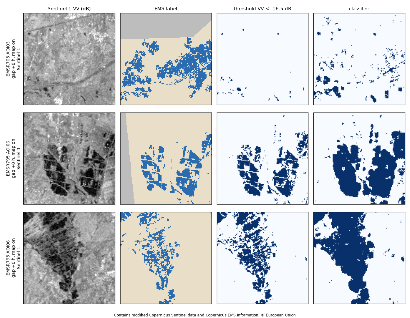
How to read them. 8 of the 24 pairs have an EMS map drawn on the same Sentinel-1 image the detectors see (gap ≈ 0 h): there the score partly measures agreement with the EMS analyst's own reading of that image, and it is good (CSI ≈ 0.39). On the labels drawn on other sensors (optical, aerial, a different date) both detectors almost fail (CSI 0.04–0.07): water under vegetation or in towns, flooding that receded or arrived between the two acquisitions, and areas mapped as flooded that radar sees as rough are not in one VV image. The headline "all" score is carried by the same-image areas; quote the split scores, not that one. The classifier, trained mostly on dry chips (1.1 % flooded), over-predicts about twice the area: class weighting, a pre-event reference scene and the DEM are the next steps, and the same split is what a foundation model has to beat.
Results of notebook 02
From workflow run 41853533004 (4 November 2026): all 24 pairs found a reference of the same relative orbit, 12 days before for 19 of them and 6 days before for 5, for 93.7 PU. The chips and the test areas are the same as in notebook 01.
| Detector | Labels | CSI | POD | FAR | F1 | bias |
|---|---|---|---|---|---|---|
| VV threshold | same image | 0.394 | 0.548 | 0.417 | 0.565 | 0.94 |
| change threshold (VV < −14 dB, ΔVV < −4 dB) | same image | 0.417 | 0.552 | 0.369 | 0.589 | 0.87 |
| classifier, one image | same image | 0.299 | 0.692 | 0.655 | 0.461 | 2.00 |
| classifier, change | same image | 0.361 | 0.763 | 0.593 | 0.531 | 1.88 |
| VV threshold | independent | 0.037 | 0.058 | 0.906 | 0.072 | 0.62 |
| change threshold | independent | 0.040 | 0.040 | 0.108 | 0.077 | 0.05 |
| classifier, one image | independent | 0.071 | 0.219 | 0.904 | 0.133 | 2.29 |
| classifier, change | independent | 0.032 | 0.196 | 0.963 | 0.062 | 5.31 |
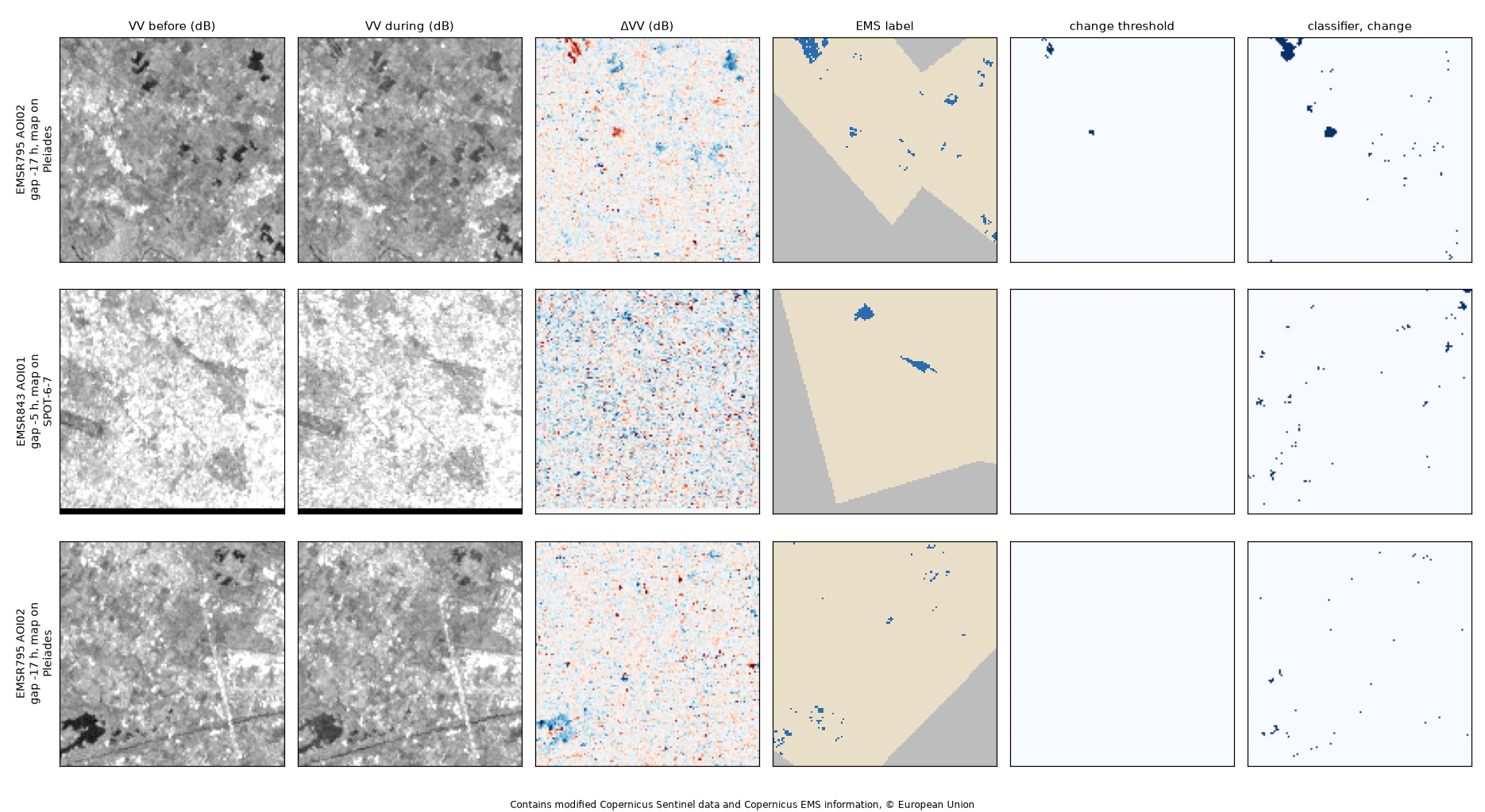
How to read them.
- Where the label shares the image, change helps. The change threshold raises CSI from 0.39 to 0.42 and cuts false alarms (FAR 0.42 to 0.37). The change classifier gains 0.06 CSI over the one-image classifier.
- On independent labels it does not help, and the figure shows why. Those test maps were drawn on Pléiades and SPOT, very-high-resolution optical images, as many small scattered polygons. At 40 m most of them are a pixel or two, and ΔVV shows hardly any change there: the water was shallow, short-lived or under cover, or it had receded in the 5–17 h between the two acquisitions. The change threshold becomes very cautious (bias 0.05, FAR 0.11): what it marks is mostly right, but it finds almost nothing.
- What would move the independent score: a finer grid (20 m or 10 m,
4–16 × the PU), keeping only pairs with a small
gap_hours, and more activations with independent maps of large floods. 28 test chips from two areas are too few to separate the models from the label type.
The notebooks are stored without outputs. Each one saves its figure in
docs/images/.
Data: Copernicus EMS Rapid Mapping, © European Union; Copernicus Sentinel-1, processed by Sentinel Hub on the Copernicus Data Space Ecosystem.